
| Master software performance in just 16 hours! Join our Software Optimization for the Memory Subsystem Workshop taking place from May 18th to May 21st. Click here to express interest or register. |
In this post we talk about how data structure data layout effects software performance and how, by modifying it, we can speed up the access and modification of the data structure. This post is a logical continuation of the previous post about class layout and performance, where we talked about how class size and class layout influences software performance.
The basic premises of good memory performance hold in this case as well:
- Everything that is accessed together should be stored together. Otherwise, the memory subsystem needs to more resources to fetch data.
- Exploite the cache line organization of the memory subsystem. Since data is brought in blocks of 64 bytes from the memory to the data caches, our programs should consume all of it.
- Keep data compact in memory speeds up access and modification. Smaller data more easily fits in the faster parts of the memory subsystem.
Techniques
Different techniques apply for different data structures. But in essence, all techniques revolve around the same idea of making the logically neighboring data physically close as well.
Polymorphism and Vectors of Pointers
In C++, to use polymorphism, you need to access the object through a pointer or a reference. And to access a collection of polymorphic objects, you need a vector of pointers (or some other data structure that holds pointers). As a data structure, a vector of pointers has two problems:
- For each pointed object there needs to be a call to a system allocator to allocate the memory for the objects.
- To access an object, a pointer needs to be dereferenced.
Many calls to the system allocator increase the memory fragmentation which can make a long running system less responsive. Additionally, pointer dereferencing often results in a cache miss, since there is zero guarantee that two neigboring pointers in the pointer array point to two neighboring objects in memory.
A solution to this problem1 involves changing the container. There are a few of them:
- Instead of vector of pointers, use a dedicated vector of objects for each type. If the objects in you array do not need to be sorted, this is the preferred way. It uses the least amount of memory, it doesn’t use polymorphism because the type of object is already known and lastly, it doesn’t make any calls to the system allocator. However, if the original vector was sorted, this property will not be maintained. The container
boost::base_collectionoffers such a data structure. - Instead of vector of pointers, use vector of
std::variant. Introduced in C++17,std::variantis a type-safe union. It can hold any of the types specified as a template parameter. For example,std::variant<circle, square, rectangle>can hold one instance of either acircle,asquareor arectangle. The amount of space consumed by a singlestd::variantis calculated as the size of the largest type in the variant, so arrays of variants consume more memory then simple vectors of pointers and dedicated vectors per type. However, compared to the previous case, vectors ofstd::variantcan be sorted. - Use polymorphic vectors. Polymorphic vector combine the advantages of polymorphism and vector of
std::variants. With polymorphic vectors, the function address is determined using virtual function mechanism, but the data is stored in the same way asstd::variant. A prototype ofpolymorphic_vectorclass can be found here. - Use vector of pointers with a custom allocator. Although this approach doesn’t avoid dereferencing pointer, we mention it here for completeness. If the vector is filled using
push_backoremplace_back, it is guaranteed that the neighboring pointers will point to the neighboring objects in memory, which will have a good effect on performance. But as the vector is modified, this may no longer be the case and the good performance of this container will be lost. Learn more about this in this post.
The advantages and disadvantages of each approach is conveniently summarized in the bellow table:
| Vector of pointers | Per type vector of objects | Vector of std::variant | Polymorphic vector | Vector of pointers with custom allocator | |
|---|---|---|---|---|---|
| Available in STL | Yes | No | Yes | No | Yes |
| Fast iteration | No | Yes | Yes | Yes | Yes initially |
| Good memory consumption | Yes | Yes | No | No | Yes |
| Avoids memory fragmentation | No | Yes | Yes | Yes | Yes |
| Preserved good performance when container modified | No | Yes | Yes | Yes | No |
| Sortable | Yes | No | Yes | Yes | Yes |
| Cheap to swap elements in vector | Yes | No | No | No | Yes |
Do you need to discuss a performance problem in your project? Or maybe you want a vectorization training for yourself or your team? Contact us
You can also subscribe to our mailing list (link top right of this page) or follow us on LinkedIn , Twitter or Mastodon and get notified as soon as new content becomes available.
Linked Lists
Linked lists as data structures are very flexible as they allow insertion and removal anywhere in the list with O(1) complexity. However, linked lists are probably the most inefficient data structure that exists from the hardware efficiency point of view. Linked lists have low instruction-level parallelism, logically neighboring nodes can be scattered all around the memory, and finally, it is difficult to use vectorization to speed up access to linked lists.
To speed up access and modification of a linked list, we can modify the linked list’s data layout. Instead of holding a value and a pointer to the next node, we hold two or more values inside a single node. Here is the graphical representation of such a linked list:
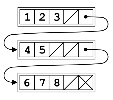
In this case, a singe linked list node contains up to four values. This kind of linked list is called unrolled linked lists and in this case the unroll factor is 4. There are several advantages of this approach:
- Better memory efficiency and better cache line utilization.
- Decreased memory fragmentation.
- If all nodes are full, they use less memory because there is only one next pointer per N values.
Of course, there are downsides as well. Insertion, traversal and other operations are more complex. Also, there is a possibility of larger memory utilization if nodes contain less than N values per node.
We measure the performance impact of such lists in the experiments section.
Binary Trees
In binary trees, each parent node has two children nodes, left and right. Left and right children are logical followers of the parent, and it is more memory efficient to keep them in the same place. There are two ways to do it: by modifying the memory layout using a custom allocator (talked about it in this post), or by modifying the binary tree node layout.
If we want to modify the binary tree data layout, one of the ways to do it is to bring the parent, the left child and the right child into a single node. By doing this, our tree node which originally contained 1 value and 2 pointers, now contains 3 values and 4 pointers. Essentially, we converted from a binary tree to a quaternary tree. Here is the how it is done graphically:

This operation increases memory efficiency because we are storing a parent and its children in a same chunk of memory. Actually, it reminds a lot of Van de Emde Boas Layout we covered in the previous post. But, compared to it, it has a huge advantage. The algorithms for insertion, deletion and modification are all well known and they preserve the property of the tree to hold more than one value in a singe node.
Generally, N-ary trees are more memory efficient than binary trees for a few reasons:
- Better memory efficiency. A single node holds more than one value, which can often belong to the same cache line.
- The tree is shallower, which means less pointer dereferences and less data cache misses.
We experiment with trees in the experiment section.
Hash Maps
The most common type of hash map is separate chaining hash map. The hash map itself is an array of buckets, and each bucket is a simple pointer to a hash map node. When we need to insert a new value into the hash map, we find its bucket, allocate a new hash map node, fill it with data and make the pointer in the bucket point to newly allocated node. If we need to insert another value to the same bucket, we allocate another hash map node and link it with the existing node. The memory layout looks like this (examples taken from Wikipedia):

When we want to access our data, the hash map applies the hash function on the key to get the location of the bucket that holds our data. Accessing a bucket is a random memory access that mostly result in a cache miss. And this cache miss is mandatory, since the hash map cannot function without it. Next, to get to the actual data, the hash map needs to dereference the pointer in the bucket. And if the key in the first hash map node isn’t the one we are looking for, it needs to dereference the chain of pointers until it finds the value it is looking for.
To improve data locality, instead of storing only the pointer in the bucket, we store one piece of useful data. If there are no collision, the hash map obtains our data with only one pointer dereference (when the access to the bucket is made). Bear in mind that this can substantially increase the size of the hash map because the empty buckets take as much space as buckets filled with one value. Here is the graphical representation of this idea:

This will work very well if the hash map has few collisions. But if the number of collisions is high, we have the same problem as earlier: dereferencing a collision chain which is essentially a linked list and related data cache misses.
A solution to this problem is another type of hash map called open addressing. Instead of storing a collided value in a separate list, it stores the collided value in the next bucket.

In this case, if we enter the bucket and the key doesn’t correspond to the key we are looking for, we can move to the next bucket, which is a neighboring memory address with a potential to be in the same cache line.
Open addressing hash maps are not without their problems however. If the load factor (percentage of used bucket) is too high, the performance may suffer because the collision chain can be long. Separate chaining hash maps are more resilient to high load factors.
We experiment with open addressing hash maps in the experiment section.
Do you need to discuss a performance problem in your project? Or maybe you want a vectorization training for yourself or your team? Contact us
You can also subscribe to our mailing list (link top right of this page) or follow us on LinkedIn , Twitter or Mastodon and get notified as soon as new content becomes available.
Experiments
In the experiments section we measuring how modifying data structure layout impacts software performance. We repeated each measurement five times and report the average numbers. The benchmarks were performed on Intel(R) Core(TM) i5-10210U system. The source code is available here. We repeat each experiment five times and report the average numbers.
Vector of Pointers
In this experiment we test the performance of vector of pointers compared to vector of std::variant. Our array has 128 M entries, and we measure the time needed to iterate it once. Source code is available here.
We perform three measurements:
- Vector of pointers in an environment with a very low memory fragmentation, essentially corresponding to an vector of pointers where logically neighboring pointers point to logically neighboring memory addresses. This happens in small test examples like this, but very rarely on long running complex programs or vectors that have been modified a lot.
- Vector of pointers in an environment with a very high memory fragmentation. We achieve this by shuffling the vector of pointers.
- Vector of
std::variant.
Here are the runtimes:
| Vector Type | Runtime |
|---|---|
| Vector of Pointers, Low Fragmentation | 0.480 s |
| Vector of Pointers, High Fragmentation | 7.995 s |
Vector of std::variant | 0.390 s |
In a low fragmentation environment, the vector of pointers is a bit slower than the vector of std::variant. However, in a high fragmentation environment, the speed difference is drastic. Dereferencing pointers to random locations in memory is a performance killer!
Unrolled Linked Lists
For linked lists test, we implemented several types of linked lists that hold 1, 2, 4 or 8 values in a single node (link to the source code). We perform the test like this:
- Insert 50000 elements in a linked list.
- Remove one quarter of the elements. Some of the nodes will contain less than an optimal number of elements.
We test how much time does it take to perform 50.000 lookups into the linked list. Since our testing environment is empty, one can expect that the allocator returns neighboring memory addresses. In a system that has been running for a long time and a linked list that has been modified a lot this will not be the case. Therefore, we test in two different environments:
- Environment with a very low memory fragmentation, essentially corresponding to a linked list where logically neighboring nodes are physical neighbors in memory. This happens in small test examples like this, but very rarely on long running complex programs or linked lists that have been modified a lot.
- Environment with a very high memory fragmentation. We achieve this by shuffling the nodes in the linked list.
Here are the runtimes for the environment with low memory fragmentation:
| Number of Values in a Node | Runtime | Instructions |
|---|---|---|
| 1 | 3.505 s | 9375 M |
| 2 | 6.951 s | 8983 M |
| 4 | 3.778 s | 7810 M |
| 8 | 3.584 s | 8400 M |
When the memory fragmentation is low, most linked lists behave in a similar manner. The linked list has an unusual spike for 2 values in a node, but upon closer inspection, we see that in this case the program makes two time more accesses to L3 cache than other test cases. This could be explained because the size of node is 48 and it is often split between two cache lines, forcing the code to perform two accesses to the L3 cache instead of one just to get two values.
Here are the same measurements, but for high memory fragmentation environment:
| Number of Values in a Node | Runtime | Instructions |
|---|---|---|
| 1 | 14.412 s | 9375 M |
| 2 | 12.269 s | 8983 M |
| 4 | 7.279 s | 7810 M |
| 8 | 5.261 s | 8400 M |
In this environment, the clear winner is the list with the largest number of values in a node.
Hash Maps
For hash maps, we compare two hash maps: a hash map with separate chaining where the first value is stored in the bucket (source code). And the second is a hash map with open addressing(source code), where, if the current bucket is occupied, we lookup a place in the following buckets.
Our hash map have fixed sizes which are compile time parameter. Additionally, the hash map size is always a power of two, which means we can cheaply calculate the bucket using masking. In addition, we measure the runtime for std::unordered_map and absl::flat_hash_map.
Since the performance of hash map depends a lot on the load factor, we keep the load factor low (about 30%). Open addressing hash maps behave badly when the load factor is high because of the way they resolve collisions. By keeping the load factor low we are actually testing memory efficiency instead of counting steps to search the collision chain.
Here are the runtimes for various types of hash maps, depending on the hash map size:
The graph shows that most hash maps are similar in performance for small hash map sizes, but once the memory subsystem becomes the bottleneck, the open addressing hash map is the fastest.
If you look at the graph, you see that there the runtime goes down for the largest hash map (32 M). This happens because the number of collisions becomes smaller. It is about 5% for 32 M separate chaining hash map compared to 25% for 4 M separate chaining.
N-ary trees
In this experiment, we measure the performance of various types of trees (source code). The number of values inside a binary node goes from 1 to 8 values in a node. We perform 10 M lookups in various tree sizes. Here are the runtimes depending on number of values in the node and tree size:
The graph is not very clear, but it displays that the general trend that the more values in a single node are typically faster than nodes with only one value, especially for very large trees that are mostly fetched from the main memory.
Here is the table for the fastest tree depending on the tree size:
| Tree Size (in values) | Values in the Node of the Fastes Tree | Speedup Compared to 1 Value in Node |
|---|---|---|
| 4K | 4 | 1.27 x |
| 16K | 4 | 1.22 x |
| 64K | 5 | 1.51 x |
| 256K | 5 | 1.29 x |
| 1M | 6 | 2.07 x |
| 4M | 8 | 2.45 x |
| 16M | 7 | 2.36 x |
The bigger the tree, the bigger the likelihood that its data will predominately be in the slower part of the memory subsystem. And slower parts of the memory subsystem profit more from binary trees with many values in a single node.
Do you need to discuss a performance problem in your project? Or maybe you want a vectorization training for yourself or your team? Contact us
You can also subscribe to our mailing list (link top right of this page) or follow us on LinkedIn , Twitter or Mastodon and get notified as soon as new content becomes available.
- This is not the only way, it is also possible to fix it using memory pools [↩]
Hi Ivica,
thanks for the great stuff you publish here. On topic of t this post, have you seen this post by Poul-Henning Kamp the author of Varnish https://queue.acm.org/detail.cfm?id=1814327 ?
He touches similar things but at a slightly higher level, i.e. virtual memory management within the OS.
Very well written and useful. Thank you for this