| Master software performance in just 16 hours! Join our Software Optimization for the Memory Subsystem Workshop taking place from May 18th to May 21st. Click here to express interest or register. |
Cache Miss Types
When a cache miss occurs, there are four reasons why this happened (called the four Cs). These are:
- Compulsory – we are accessing a piece of data for the first time, so by definition we have a cache miss.
- Capacity – we are accessing a piece of data which was earlier already in the cache, but got evicted because the cache was too small and the place was needed for some other data.
- Conflict – happens when two different pieces of data contend for the same line in the data cache. So the newer data will kick out the older data.
- Coherency – happens in a multicore environment, when the same piece of data cached by core 1 is modified by core 2. In some implementations, the data cached by core 1 will be evicted.
Out of all cache miss types, only compulsory cannot be avoided. For other types, we can decrease their frequency or completely avoid them, depending on the circumstances. We covered this in many of our earlier articles. For software optimizations, it can be useful to know what kind of cache miss type is happening in our programs.
Throughput Bound VS Latency Bound
If a loop of interest is memory bound, this means it has some kind of bottleneck in the memory subsystem. There are two basic types of memory subsystem bottlenecks:
- Throughput bottleneck – happens when a certain part of the memory subsystem (main memory, L1 cache, etc) is reaching its maximum throughput (throughput is often measured in GB/s). In order to speed up the loop, we would need to figure out to decrease the pressure on that part of the memory subsystem.
- Latency bottleneck – normally, a CPU core might be executing hundreds of instructions simultaneously, in various phases of execution. This allows it to hide access latency to the memory subsystem – while the CPU core is waiting for data for a load instruction, it is can execute other instructions. However, certain types of codes do not allow this. When this is the case, the CPU is mostly idle and waits for the data from the memory subsystem. The performance of such codes directly depends on the memory subsystem’s latency, which is the time between when the request is issues and request is served.
Top-Down Microarchitectural Analysis
Top-Down Microarchitectural Analysis (TDMA) allows you to analyze your source code functions for hardware inefficiencies. It will measure what percentage of CPU pipeline slots1 is wasted because the CPU was unable to fill them because of hardware inefficiencies.

All pipeline slots are categorized into our groups: Retiring, Bad Speculation, Front-End Bound and Back-End-Bound. Only slots in the Retiring category are efficiently utilized, and the goal is to have the largest percentage of slots in this category.
Memory bound programs will have the largest percentage of wasted slots in Back-End-Bound category, and more specific, in Memory Bound subcategory.
Tools that support this methodology are Intel’s VTUNE profiler, PMU-tools and ARM MAP. There is no tool for AMD processors that supports TDMA, but luckily, if a program is memory bound on Intel’s CPU, it will be almost certainly memory bound on AMD’s CPU as well. We will not describe how to use these tools, for this refer to their documentation.
Here is an output of Intel’s VTUNE on one of our test code:

As you can see, the memory bound category is further split into L1 bound, L2 bound, L3 bound, DRAM bound and Store bound. You can read about the meaning of each individual subcategory by hovering the mouse over its name.
The columns with largest percentages represent hardware parts where you should focus your optimization efforts, because you can expect the most improvements.
Do you need to discuss a performance problem in your project? Or maybe you want a vectorization training for yourself or your team? Contact us
You can also subscribe to our mailing list (link top right of this page) or follow us on LinkedIn , Twitter or Mastodon and get notified as soon as new content becomes available.
Roofline Model and Arithmetic Intensity
First let’s explain what arithmetic intensity is. Consider the following loop:
for (int i = 0; i < n; i++) {
    out[i] = a[i] + b[i];
}
Per iteration, this loop:
- Reads 2 integers (
a[i]andb[i]). - Performs one addition.
- Writes one integer (
out[i]).
The ratio between number of operations (floating point operations FLOP or integer operations IOP) and number of bytes transferred between the core and the memory subsystem is called arithmetic intensity. In this example, there is one operation per 12 bytes of access, so the arithmetic intensity is 1 / 12 = 0.083. Arithmetic intensity is a property of each a loop and it is hardware independent.
Additionally, we need to introduce two terms related to peak hardware performance:
- Peak floating-point operation per second (FLOPS) and peak integer operations per second (IOPS) are two measurements for maximum achievable operations per second. This is the upper limit on the rate of which the architecture can crunch numbers, when all conditions are favorable.
- Peak L1 data throughput, peak L2 data throughput, peak L3 data throughput and peak memory throughput (in GB/s). This is the upper limit on the rate the architecture can supply numbers to the core.
Both of these numbers are property of the architecture. Faster architecture have better numbers.
Scientists have determined that there is a dependency between arithmetic intensity, maximum data throughput and maximum OPS. This dependency looks like this (image source):
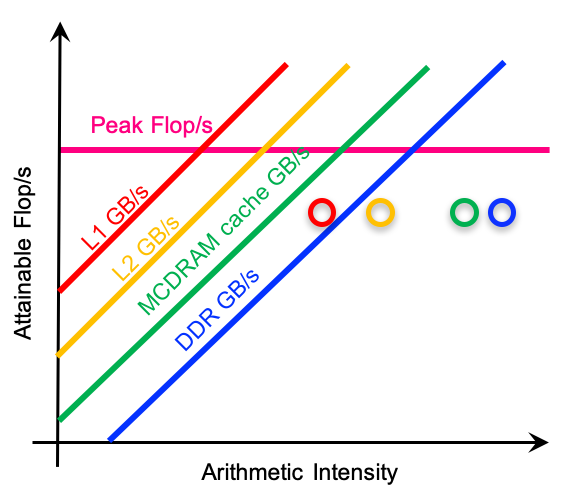
This graph is called the roofline graph. It shows that peak achievable OPS depends on both arithmetic intensity and peak memory subsystem throughput. And the peak OPS is smaller for loops with arithmetic intensity. In order words, loops with smaller arithmetic intensity are more often memory bound, and loops with a higher arithmetic intensity are more often core bound.
We can use the roofline graph to check if a loop is using hardware efficiently. To do this, we first calculate its arithmetic intensity, either manually or by measuring it. Also, we calculate its OPS rate, again either manually or by measuring it. These two numbers represent a dot in the roofline graph. We created the roofline graph for our three test loops using Intel’s ADVISOR:

Three dots in the graph represent measured OPS for three functions matrix_mul1, matrix_mul2 and matrix_mul3. The red dot represents matrix_mul2, which experiences cache conflicts and it is dominantly fetching data from memory. On the other hand, matrix_mul1 and matrix_mul2 are above the DRAM bandwidth roofline. These implementations are not particularly efficient, since matrix multiplication can be made to reach the L1 roofline bandwidth.
There are two ways to draw the roofline graph:
- Intel’s Advisor can do all the measurements and graph drawing automatically.
- You can measure peak OPS and data throughput using LIKWID and draw the graph manually. The instruction is here.
Cache-Miss Metrics
Cache miss related metrics are a number one indications of problems fetching data from the memory subsystem. It can indicate both memory throughput and memory latency problem. Also, it happens for all four types of cache misses: compulsory, capacity, conflicts and coherency.
There are in total three cache-miss metrics (LX can be L1, L2 or L3):
- LX request rate – number of LX cache requests per instruction. If the request rate is low, the data is being fetched from the faster parts of the memory subsystem (cache L(X-1) ). For example, if L2 request rate is low, that means that the data is mostly fetched from the L1 cache.
- LX miss rate – number of LX cache misses per instruction. If the request rate is high but the miss rate is low, that means that the data is mostly fetched from the cache LX. If the miss rate is high, the data is mostly fetched from the slower parts of the memory subsystem (cache L(X + 1) or memory).
- LX miss ratio – ratio between LX cache misses and LX cache requests. This is the most commonly cited metric in the literature, but it is only meaningful if LX request rate is high.
These three metrics allows us to understand quickly from which part of the memory subsystem does the bulk of our data come.
We can use LIKWID to collect information measure request rates, miss rates and miss ratio for L2 and L3 caches on most architectures. You can find more information on how to enable LIKWID and how to set up a marker API to measure counters for your segment of code here.
We ran LIKWID on one of our test programs from a previous post. We had a small kernel like this:
for (int i = 0; i < n; i++) {
    out[i] = a[i] + b[i];
}
To run the test, surround your code with LIKWID_MARKER_START and LIKWID_MARKER_STOP calls, recompile your program with LIKWID, and then from the command line execute:
# For L2 cache misses
$ likwid-perfctr -g L2CACHE -m -C 0 ./my_app

# For L3 cache misses
$ likwid-perfctr -g L3CACHE -m -C 0 ./my_app
We repeat the experiments for various array sizes. Here are the numbers for the most interesting array sizes:
| Array Size (elements2 ) | Runtime (s) | L2 Request Rate | L2 Miss Rate | L2 Miss Ratio | L3 Request Rate | L3 Miss Rate | L3 Miss Ratio |
|---|---|---|---|---|---|---|---|
| 4K | 0.094484 | 0.7988 | 0.0001 | 0.0001 | 0 | 0 | 0.0177 |
| 8K | 0.09965 | 1.0272 | 0.1381 | 0.1345 | 0.0096 | 0 | 0 |
| 16K | 0.120721 | 1.5241 | 0.4516 | 0.2963 | 0.0315 | 0 | 0 |
| 32K | 0.142315 | 1.7381 | 0.5871 | 0.3378 | 0.0425 | 0 | 0 |
| 64K | 0.145207 | 1.7386 | 0.5857 | 0.3369 | 0.0427 | 0 | 0 |
| 128K | 0.139029 | 1.7393 | 0.5876 | 0.3378 | 0.0429 | 0.0004 | 0.0103 |
| 256K | 0.195931 | 1.8598 | 0.6284 | 0.3379 | 0.0486 | 0.0081 | 0.1664 |
| 512K | 0.288241 | 1.9483 | 0.6626 | 0.3401 | 0.0542 | 0.0121 | 0.2234 |
| 1024K | 0.334989 | 1.9775 | 0.6593 | 0.3334 | 0.0696 | 0.0238 | 0.3421 |
Even for the smallest array size, the data is mostly served from L2 cache (high L2 request rate). As the array size grows, so does L2 miss rate. For the array size of 8K, we see some L2 cache misses which continue to grow. Starting from the array size of 16K, the data starts to be fetched from L3 cache as well. And starting from the array size 512 K, we start to notice L3 cache misses as well.
Do you need to discuss a performance problem in your project? Or maybe you want a vectorization training for yourself or your team? Contact us
You can also subscribe to our mailing list (link top right of this page) or follow us on LinkedIn , Twitter or Mastodon and get notified as soon as new content becomes available.
Data Throughput
Data throughput is the amount of traffic per second transferred between one part of the memory subsystem and the CPU core. It is typically measured in MB/s or GB/s. For us performance engineers, data throughput is interesting if we want to see if a hot loop is consuming all the available hardware data bandwidth.
We can collect throughput data using LIKWID as well. The names of performance groups are L2, L3 and MEM. To collect them, execute:
# For L2 throghout
$ likwid-perfctr -g L2 -m -C 0 ./my_app

# For L3 throughput
$ likwid-perfctr -g L3 -m -C 0 ./my_app

# For memory throughput
$ likwid-perfctr -g MEM -m -C 0 ./my_app
There are two metrics related to data throughput:
- Load Bandwidth – the data volume per time leaving LX cache or memory and going to the faster parts of the memory subsystem or the CPU.
- Evict Bandwidth – the data volume per time arriving to LX cache or memory from the faster parts of the memory subsystem or the CPU.
To illustrate data throughput, we use the same example as in the previous section. Here are the measured numbers:
| Array Size | L2D Load Bandwidth (MB/s) | L2D Evict Bandwidth (MB/s) | L3D Load Bandwidth (MB/s) | L3D Evict Bandwidth (MB/s) | MEM Load Bandwidth (MB/s) | MEM Evict Bandwidth (MB/s) |
|---|---|---|---|---|---|---|
| 4 K | 55818.8902 | 18541.4908 | 9373.3586 | 4931.3925 | 690.5863 | 4.121 |
| 8 K | 65800.6705 | 21959.1913 | 9646.6656 | 3279.6959 | 716.858 | 6.382 |
| 16 K | 50143.9794 | 16725.1599 | 43265.5648 | 14927.8941 | 722.4256 | 10.1824 |
| 32 K | 43475.5863 | 14437.1153 | 46419.2204 | 15677.8174 | 678.804 | 2.6182 |
| 64 K | 46275.0098 | 15364.0398 | 44408.1247 | 14875.3722 | 687.9786 | 5.2899 |
| 128 K | 45429.8501 | 15084.1242 | 46449.1278 | 15742.1058 | 1420.5126 | 228.0579 |
| 256 K | 31266.2653 | 10382.0743 | 31937.4242 | 15903.4359 | 9260.1124 | 2667.5343 |
| 512 K | 23682.3741 | 7866.7263 | 24626.9151 | 18280.7016 | 15432.6815 | 4388.6026 |
| 1 M | 18652.6192 | 6204.8379 | 19020.8461 | 16984.8759 | 16415.1153 | 4959.9227 |
| 2 M | 18356.4865 | 6095.7787 | 17997.084 | 17127.6113 | 17413.5186 | 5429.7742 |
In the example above, peak measured L2D load bandwidth of 65800.6705 MB/s is achieved for array size 8 K, peak measured L3D bandwidth of is achieved for array size 46449.1278 for array size of 128 K, and peak measured memory load bandwidth of 17413.5186 MB/s is achieved for array size of 2 M.
Cache-miss rate alone is not a reliable indicator if a loop is throughput bound. A loop with a high arithmetic intensity can have a lot of cache misses and yet not be memory throughput bound but core bound. Only if our loop is reaching peak data throughput at cache LX or memory is our loop actually throughput bound. One tool that can be used to measure the peak data throughput is likwid-bench. If a program is not reaching the peak data throughout, it is either memory latency bound or core bound.
Data Volume
Data volume measures the amount of data transferred between the memory subsystem and the CPU core. Typically it is measured in GB. We can use LIKWID’s performance groups L2, L3 and MEM to measure data volume our code is consuming or producing. Here is how to collect the data:
# For L2 throghout
$ likwid-perfctr -g L2 -m -C 0 ./my_app

# For L3 throughput
$ likwid-perfctr -g L3 -m -C 0 ./my_app

# For memory throughput
$ likwid-perfctr -g MEM -m -C 0 ./my_app
There are two metrics related to data volume:
- Load Volume – the data volume leaving LX cache or memory and going to the faster parts of the memory subsystem or the CPU.
- Evict Volume – the data volume arriving to LX cache or memory from the faster parts of the memory subsystem or the CPU.
And here is the output for our test program that we have been using in the last two sections:
| Array Size | L2D Load Volume (GB) | L2D Evict Volume (GB) | L3D Load Volume (GB) | L3D Evict Volume (GB) | MEM Load Volume (GB) | MEM Evict Volume (GB) |
|---|---|---|---|---|---|---|
| 4 K | 6.5044 | 2.1606 | 0.9695 | 0.5101 | 0.0674 | 0.0004 |
| 8 K | 6.4535 | 2.1537 | 0.8158 | 0.2773 | 0.0717 | 0.0006 |
| 16 K | 6.4479 | 2.1507 | 5.1841 <- | 1.7887 | 0.0927 | 0.0013 |
| 32 K | 6.4716 | 2.149 | 6.4674 | 2.1843 | 0.0977 | 0.0004 |
| 64 K | 6.4704 | 2.1483 | 6.4641 | 2.1653 | 0.0982 | 0.0008 |
| 128 K | 6.4691 | 2.1479 | 6.4595 | 2.1892 | 0.2242 | 0.036 |
| 256 K | 6.4674 | 2.1475 | 6.4643 | 3.2189 | 1.8856 | 0.5432 |
| 512 K | 6.4698 | 2.1491 | 6.4687 | 4.8018 | 4.1853 <- | 1.1902 |
| 1 M | 6.4557 | 2.1475 | 6.469 | 5.7766 | 5.6305 | 1.7013 |
| 2 M | 6.4666 | 2.1474 | 6.4692 | 6.1567 | 6.2973 | 1.9636 |
Measuring data volume is useful because it can be compared to manually calculated data volume to check for inefficiencies. If manually calculated data volume and the measured value do not correspond, this can indicate problems in the memory subsystem (typically cache line not being used fully for various reasons).
In our example, the total data volume loaded is sizeof(double) x ITERATION_COUNT x 2 = 8 x 256 M x 2 = 4 GB. And the total data volume stored is sizeof(double) x ITERATION_COUNT x 1 = 2 GB. However, if we look the above table, we measured 6 GB of data reads. This is because storing data to memory consists of of reading a cache line, modifying it, then storing it back. This can be fixed by using streaming loads instead of regular loads.
TLB Cache Misses
We can measure TLB cache miss rate using TLB_DATA performance group in LIKWID. Here is the LIKWID output for the random memory access example:
$ likwid-perfctr -g TLB_DATA -m -C 0  ./memory_throughput

...

+-----------------------------------+--------------+
|               Metric              |  HWThread 0  |
+-----------------------------------+--------------+
|        Runtime (RDTSC) [s]        |       4.2040 |
|        Runtime unhalted [s]       |       1.0763 |
|            Clock [MHz]            |     543.7881 |
|                CPI                |      14.4515 |
|        L1 DTLB load misses        |     65620510 |
|       L1 DTLB load miss rate      |       0.4172 |
|  L1 DTLB load miss duration [Cyc] |      34.4261 |
|        L1 DTLB store misses       |            7 |
|      L1 DTLB store miss rate      | 4.450336e-08 |
| L1 DTLB store miss duration [Cyc] |      55.5714 |
+-----------------------------------+--------------+
The L1 DTLB load miss rate (misses per instruction) is very high, 0.4172. Rerunning the same test with huge pages enabled results in much better numbers:
$ TCMALLOC_MEMFS_MALLOC_PATH=/dev/hugepages/tcmalloc LD_PRELOAD=/usr/lib/x86_64-linux-gnu/libtcmalloc_minimal.so.4  likwid-perfctr -g TLB_DATA -m -C 0  ./memory_throughput

...

+-----------------------------------+--------------+
|               Metric              |  HWThread 0  |
+-----------------------------------+--------------+
|        Runtime (RDTSC) [s]        |       1.5144 |
|        Runtime unhalted [s]       |       0.5353 |
|            Clock [MHz]            |     748.6865 |
|                CPI                |       7.1864 |
|        L1 DTLB load misses        |          218 |
|       L1 DTLB load miss rate      | 1.385970e-06 |
|  L1 DTLB load miss duration [Cyc] |      78.4954 |
|        L1 DTLB store misses       |            0 |
|      L1 DTLB store miss rate      |            0 |
| L1 DTLB store miss duration [Cyc] |       -      |
+-----------------------------------+--------------+
Do you need to discuss a performance problem in your project? Or maybe you want a vectorization training for yourself or your team? Contact us
You can also subscribe to our mailing list (link top right of this page) or follow us on LinkedIn , Twitter or Mastodon and get notified as soon as new content becomes available.
False Sharing
False sharing can also be detected using LIKWID. For our false sharing example, performance output looks like this:
$ sudo likwid-perfctr -m -g FALSE_SHARE -C 0-3 ./multithreading

...

+---------------------------------+------------+------------+------------+------------+
|              Metric             | HWThread 0 | HWThread 1 | HWThread 2 | HWThread 3 |
+---------------------------------+------------+------------+------------+------------+
|       Runtime (RDTSC) [s]       |     0.3870 |     0.2823 |     0.4367 |     0.4396 |
|       Runtime unhalted [s]      |     0.3852 |     0.2764 |     0.4283 |     0.4398 |
|           Clock [MHz]           |  2209.3023 |  2135.6685 |  2176.1156 |  2216.7725 |
|               CPI               |     5.6427 |     4.0486 |     6.2740 |     6.4416 |
| Local LLC false sharing [MByte] |     8.9804 |     4.9166 |    12.9420 |    13.2354 |
|   Local LLC false sharing rate  |     0.0018 |     0.0010 |     0.0026 |     0.0026 |
+---------------------------------+------------+------------+------------+------------+
We see here false sharing rates for each thread (total of 4 threads). They do not look large, but the ideal value for false sharing rate is zero. Here is the LIKWID output after we have fixed the false sharing problem:
+---------------------------------+--------------+------------+--------------+--------------+
|              Metric             |  HWThread 0  | HWThread 1 |  HWThread 2  |  HWThread 3  |
+---------------------------------+--------------+------------+--------------+--------------+
|       Runtime (RDTSC) [s]       |       0.0808 |     0.1002 |       0.0983 |       0.0825 |
|       Runtime unhalted [s]      |       0.0964 |     0.0963 |       0.0966 |       0.0968 |
|           Clock [MHz]           |    2585.1357 |  2077.4923 |    2126.7071 |    2541.5551 |
|               CPI               |       1.4124 |     1.4104 |       1.4148 |       1.4175 |
| Local LLC false sharing [MByte] |       0.0006 |          0 |       0.0001 |       0.0001 |
|   Local LLC false sharing rate  | 1.271538e-07 |          0 | 1.271547e-08 | 1.271544e-08 |
+---------------------------------+--------------+------------+--------------+--------------+
Both runtimes and false sharing rates have become much better.
False sharing is related to coherency misses, when modification of data by one CPU core causes an invalidation of the whole cache line in another CPU core.
NUMA accesses
It is also possible to measure accesses to non-local memory for NUMA systems. The name of the performance group in LIKWID is NUMA. Unfortunately, we didn’t have a NUMA system at our disposal so we couldn’t test it.
What cannot be measured?
There are a few things that would be interesting to measure, but this is not possible with the current state of technology:
- Detecting Cache Conflicts – there is no reliable way to detect cache misses that are due to cache conflicts.
- Prefetcher Statistics – it would be interesting to see the prefetcher statistics about the number of times the prefetcher got activated divided by number of memory accesses.
Final Words
Measuring is useful to confirm our suspicions about what is going on with our software. Here we only covered the basics of memory performance measurements, but having this numbers will help you understand why your code is memory inefficient, and the rest of tips from this blog, to improve its performance.
We have seen a few times where the tools are producing numbers that do not make sense. On some architectures, some counters can be broken on unreliable. So always take the results with a grain of salt.
Do you need to discuss a performance problem in your project? Or maybe you want a vectorization training for yourself or your team? Contact us
You can also subscribe to our mailing list (link top right of this page) or follow us on LinkedIn , Twitter or Mastodon and get notified as soon as new content becomes available.